eFatigue gives you everything you need to perform state-of-the-art fatigue analysis over the web. Click here to learn more about eFatigue.
Multiaxial Strain-Life Technical Background
Fatigue occurs on the surface where one of the principal stresses is usually zero. As a result, multiaxial fatigue problems are usually biaxial in nature. Here we have assumed that the stress normal to the free surface is zero in all the calculations. Any stress concentration effects must be included in the input loading data.
Strain life analysis can be summarized as a series of steps:
- define applied stresses or strains
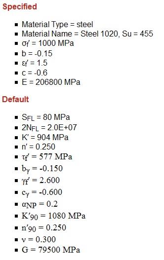
- select material properties
- compute local stresses and strains
- compute fatigue damage
- search for possible failure planes
Go to the Constant Amplitude Technical Background section for a more complete description of the fatigue variables.
Loading
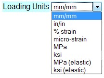
First, loading units must be specified. You can select either stress or strain units from the list.
Stress and strain simulation is an integral part of any multiaxial strain-life analysis. Loads are typically entered as strains and the corresponding stresses calculated. Stresses may also be entered and the strains will be calculated. A special entry (elastic) is used to evaluate situations where the stresses have been computed from elastic assumptions such as an elastic finite element model. In this case, the cyclic plasticity model will use the elastic input to estimate the real elastic-plastic stresses and strains.
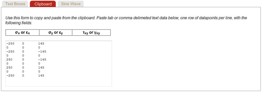
Loading histories can be entered in a series of text boxes, from the clipboard or as sine waves by selecting the appropriate tab. The individual points are connected with straight lines to obtain the loading history. If the second column is left blank, the stress σy is assumed to be zero. The stress is assumed zero even when the other columns have been entered as strain.
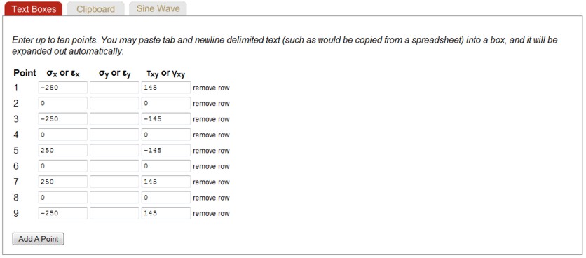
You can view the history with the Plot function. The input data shown above generated the following loading histories. Stresses as a function of time are displayed on the top row. Cross plots between the various stresses are shown in the second row.
Data entered in text boxes is also available on the Clipboard tab. In this mode, data can be copied from the clipboard or pasted to the clipboard.
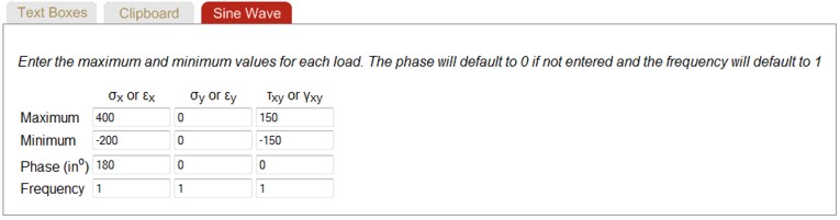
Loading histories may also be entered as a series of sine waves. The default frequency is 1 and the default phase is 0o. The frequency is a relative frequency between the various stresses or strains. Here is an example.
Cyclic Plasticity Model
One
of the more successful incremental multiaxial cyclic plasticity models has been
proposed by Jiang and Sehitoglu (Jiang and Sehitoglu "Modeling of Cyclic
Ratcheting Plasticity, Part I: Development of Constitutive
Equations," Journal of Applied Mechanics, Vol. 63, 1996,
720-725). A brief description is given here. The model is best
described in deviatoric stress space,  .
.
Yield Function
The Mises yield function, F, is expressed as

Here the notation
 is used for the deviatoric stress tensor,
 is the backstress tensor and k is the yield stress is simple shear.
Flow Rule
The normality rule is given by
where  is the exterior unit normal to
the yield surface at the loading point as defined below.
is the exterior unit normal to
the yield surface at the loading point as defined below.
Hardening Rule
The total backstress
is divided into M parts

The evolution of the backstress for each of the parts is given by
where dp is the equivalent plastic strain increment and ci, ri, and Xi are three sets of non-negative and single valued scalar functions and
Material memory is contained in the α terms. The plastic modulus function, H, is derived from the consistency condition which requires that the stress state be on the yield surface when plastic deformation is occurring.
There are four material parameters in this model, c, r, X, and k. All of these constants are computed from the cyclic stress strain curve of the material. A simple power function is fit to this curve to obtain three material properties; cyclic strength coefficient, K', cyclic strain hardening exponent, n', and elastic modulus, E.
The
shear yield strength, k, is obtained by setting the plastic strain to 0.002
(0.2%) and dividing by
 .
Both c and r are
obtained by selecting a series of stress strain pairs along the material cyclic
stress strain curve and describe the shape of the curve. Ratcheting rate is
controlled by X which is set at a fixed value of 5.
.
Both c and r are
obtained by selecting a series of stress strain pairs along the material cyclic
stress strain curve and describe the shape of the curve. Ratcheting rate is
controlled by X which is set at a fixed value of 5.
Nonproportional Hardening
Nonproportional hardening is the term used to describe loading paths where the principal strain axes rotate during cyclic loading. The simplest example would be a bar subjected to alternating cycles of tension and torsion loading. Between the tension and torsion cycles the principal axis would rotate 45°. Out-of-phase loading is a special case of nonproportional loading and is used to denote cyclic loading histories with sinusoidal or triangular waveforms and a phase difference between the loads.
Materials show additional cyclic hardening during this type of loading that is not found in uniaxial or any proportional loading path. Here is an example for 90° out-of-phase tension-torsion loading.
a) Stresses
b) Strains
This data can be converted to effective stresses and strains to obtain a stress-strain curve for nonproportional loading. Also shown is the effective stress-strain curve for the same material under proportional or in-phase loading.
The 90° out-of-phase loading path has been found to produce the largest degree of nonproportional hardening. The magnitude of the additional hardening observed for this loading path as compared to that observed in uniaxial or proportional loading is highly dependent on the microstructure and the ease with which slip systems develop in a material. A nonproportional hardening coefficient, α, can be introduced which is defined as the ratio of equivalent stress under 90° out-of-phase loading / equivalent stress under proportional loading at high plastic strains in the flat portion of the stress-strain curve. This term reflects the maximum degree of additional hardening that might occur for a given material.
The degree of nonproportionality, C, is a fourth ranked tensor which is a function of the plastic strain and the direction of the plastic strain increment.
The amount of nonproportional hardening is computed from Tanaka's parameter. (Tanaka, E., "A Nonproportionality Parameter and a Cyclic Viscoplastic Constitutive Model Taking into Account Amplitude Dependences and Memory Effects of Isotropic Hardening," European Journal of Mechanics, A/Solids, Vol. 13, 1994, 155-173).
For
any proportional loading A=0 and for 90° out-of-phase loading
 . The
material constants ri and the yield stress k are related to the nonproportional
hardening parameter in the following form,
. The
material constants ri and the yield stress k are related to the nonproportional
hardening parameter in the following form,
with two additional material constants Np and b. Np is directly related to a.
The rate of hardening is controlled by the constant b. Since we are interested in the stable solution for fatigue calculations, b = 5 is selected for numerical stability.
These
equations are now sufficient to solve for the stresses and strains under any
arbitrary loading path. The solution now proceeds by incrementally solving
these equations. The may be solved in either stress,
 ,
or strain control
,
or strain control
 .
The initial
conditions are that the stress
and backstress
start at
.
The initial
conditions are that the stress
and backstress
start at
 .
All material constants start at
their initial values as well and are updated after each loading increment.
.
All material constants start at
their initial values as well and are updated after each loading increment.
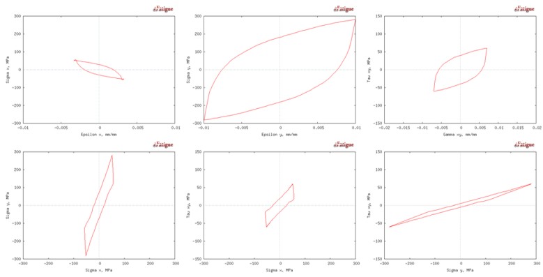
All of the cyclic plasticity models work reasonably well for proportional loading without mean stresses. Histories with combined cyclic torsion and static axial mean stresses cause problems for many models and the solution is unstable. An example of such a loading history is shown below.
Strain history and computed stresses
Axial strains are shown on the horizontal axis and shear strains on the vertical one. A static axial strain is combined with a cycle of shear strain and unloaded back to zero strain. Then an axial strain cycle is combined with a static shear strain. The loading history is repeated in compression. This loading history involves nonproportional hardening, ratcheting and stress relaxation leading to the complex stress response shown in the figure. The stresses were computed from the Jiang and Sehitoglu plasticity model described above. Six loading cycles are shown before the stress response stabilizes. Individual stress-strain response for the axial and shear loading is shown below.
Computed axial and shear stress-strain response
One good way to judge a plasticity model is to use the same model in both stress and strain control. That is, use the model to estimate the stress history from the input strains. Then use these computed stresses as input to a stress controlled version of the same model and make an estimate of the strains. The output strains of the stress controlled model should be identical to the input strains to strain controlled model. Results of this procedure for the Jiang and Sehitoglu model are given here and agreement with the original strain input data is excellent.
Computed strain history
Pseudo Stress and Strain
In uniaxial loading approximate solutions such as Neuber's rule are used to compute the stresses and strains during plastic deformation. Unfortunately, Neuber's rule cannot be directly extended to multiaxial loading because there are six unknowns and only five equations.
To overcome this problem Koettgen et al. (Koettgen V.B., Barkey M.E., and Socie, D.F. "Pseudo Stress and Pseudo Strain Based Approaches to Multiaxial Notch Analysis" Fatigue and Fracture of Engineering Materials and Structures, Vol. 18, No. 9, 1995, 981-1006) proposed a structural yield surface to obtain local elastic-plastic stresses and strains. Having defined a "yield surface," standard cyclic plasticity methods can be used to solve for the unknown stresses and strains at the notch. The material memory effects are built directly into standard cyclic plasticity calculations. The method is based on the same concept at the analytical or experimental nominal stress - notch strain curves used in uniaxial fatigue analysis such as the one shown here.
Nominal stress - notch strain curve
Cyclically, nominal stress - notch root strain response has all the features associated with stress-strain response such as hysteresis, memory, cyclic hardening and softening.
Next we introduce the concept of pseudo stress. The pseudo stress, es, or strain, ee, is defined as the theoretical elastic stress or strain computed using elastic assumptions. Neuber's rule may be written in terms of pseudo stress as follows.


These concepts can be generalized to three dimensional stress and strain states with a structural yield surface at a notch. Having defined a "structural yield surface," standard cyclic plasticity methods can be used to solve for the unknown stresses and strains at the notch. For multiaxial loading, the total stress or strain is obtained by superposition of the individual load cases.
A relationship between pseudo stress and notch strain is described with a power function that has the same form as a stress-strain curve
where the constants K* and n* represent the behavior of the structure rather than the material. Uniaxial Neuber's rule can be employed to establish the constants E*, K* and n*.
For plane stress on the surface, eσz, eτyz and eτxz are all zero and this yield function can be written as
This equation defines a structural yield function, Fo, which has the same form as the yield functions used in the plasticity models for stress-strain calculations, i.e. a Mises yield function in terms of pseudo stress.

The process may be summarized as follows:
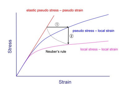
- uniaxial Neuber's rule to get K* and n*
- 1. cyclic plasticity model in stress control with pseudo constants K* and n* to obtain the pseudo stress-local strain response
- 2. cyclic plasticity model in strain control with material constants K and n to obtain the local strain - local stress response.
Damage Models
Critical plane approaches have evolved from experimental observations of the nucleation and growth of cracks during loading. Depending on the material, stress state, environment and strain amplitude, fatigue life will usually be dominated either by microcrack growth along shear planes or along tensile planes. Critical plane models incorporate the dominant parameters governing either type of crack growth. Due to the different possible failure modes, shear or tensile dominant, no single damage model should be expected to correlate test data for all materials in all life regimes. There is no consensus yet as to the best damage model to use for multiaxial fatigue life estimates and several models are included in the FatigueCalculator. Two models based on tensile strains, Smith Watson Topper and Liu Tensile and three models based on shear strains, Brown Miller, Fatemi Socie and Liu Shear are included.
Smith, Watson, and Topper
A damage model is needed for materials that fail predominantly by microcrack growth on planes of maximum tensile strain or stress, for example, cast iron, very high strength steels or 304 stainless steel under some local histories. In these materials, cracks nucleate in shear, but fatigue life is controlled by crack growth on planes perpendicular to the maximum principal stress and strain as illustrated below. Both strain range and maximum stress determine the amount of fatigue damage.
Tensile crack growth
Smith et al. (Smith, R.N., Watson, P., and Topper, T.H., "A Stress-Strain Parameter for the Fatigue of Metals," Journal of Materials, Vol. 5, No. 4, 1970, 767-778 proposed a suitable relationship that includes both the cyclic strain range and the maximum stress. This model, commonly referred to as the SWT parameter, was originally developed and continues to be used as a correction for mean stresses in uniaxial loading situations. The SWT parameter is used in the analysis of both proportionally and nonproportionally loaded components for materials that fail primarily due to mode I tensile cracking. The SWT parameter for multiaxial loading is based on the principal strain range, Δε1 and maximum stress on the principal strain range plane, σn,max.
The stress term in this model makes it suitable for describing mean stresses during multiaxial loading and nonproportional hardening effects.
Liu
Liu's (Liu, K.C., "A Method Based on Virtual Strain-Energy Parameters for Multiaxial Fatigue Life Prediction," Advances in Multiaxial Fatigue, ASTM STP 1191, D.L. McDowell and R. Ellis, Eds., American Society for Testing and Materials, Philadelphia, 1993, 67-84) virtual strain energy (VSE) model is a straight forward generalization of a uniaxial energy based fatigue life prediction model. It includes both an elastic and plastic part. Liu's model can be considered as a critical plane model since the work quantities are defined for specific planes within the material.
The virtual strain energy quantity on a plane, ΔW, is divided into elastic and plastic work components. Elastic work, ΔWe, is the sum of the two darker shaded regions in the figure while the plastic work, ΔWp, is approximated as the product, ΔσΔεp.
Elastic and Plastic Strain Energies
From the total strain life relationship it can be shown that ΔW is equal to


For multiaxial loading, the VSE model considers two possible failure models. A mode for tensile failure, ΔWI, and a mode for shear failure, ΔWII. Failure is expected to occur on the plane in the material haing the maximum VSE quantity. ΔWI is computed by first identifying the plane on which the tensile work is maximized and then adding the shear work on that same plane. Similarly, ΔWII is computed by first identifying the plane on which the shear work is maximized and then adding the tensile work component.


Here the subscript max indicates the maximum value over all planes of the quantity in the parentheses.
Liu's parameter was not originally formulated to include mean stress. One of the major effects of a mean stress on small microcracks is to alter the amount of crack closure. The amount of closure and its effect on fatigue life in mode I and mode II will be different since they do not have the same crack growth mechanism. A mean stress correction can easily be added to each of Liu's models.
It is written in terms of the stress ratio, R, to be consistent with other crack growth and closure models. This form is selected because it is the same as the SWT parameter for uniaxial loading. No fatigue damage should be computed when σn,max is less than 0. Experiments have shown that cracks are fully open for R > 0.7 and no additional mean stress effects would be expected for higher stress ratios.
In mode I, a static tensile stress in the absence of a cyclic tension stress is not damaging. But in mode II shear crack growth, a static tension will influence the crack closure forces and fatigue life. The limited amount of test data on the effect of static tension on alternating torsion suggest a linear dependence of the alternating shear stress on static tensile stress. The following formulation captures this dependence and is similar to a Goodman diagram.
Brown and Miller
Brown and Miller (Brown, M.W., and Miller, K.J., "A Theory for Fatigue Under Multiaxial Stress-Strain Conditions," Proceedings of the Institute of Mechanical Engineers, Vol. 187, 1973, 745-756) reviewed much of the available multiaxial low cycle fatigue literature with particular emphasis on the formation and early growth of microcracks. Unlike octahedral shear stress which, in some cases, has been shown to be effective when correlating high cycle fatigue failure, octahedral shear strain and maximum shear strain are not effective in describing low cycle fatigue. They conducted combined tension and torsion tests with a constant shear strain range. The normal strain range on the plane of maximum shear strain will change with the ratio of applied tension and torsion strains. Based on the data shown below for a constant shear strain amplitude, they concluded that two strain parameters are needed to describe the faigue process because the combined action of shear and normal strain reduces fatigue life.
Influence of Normal Strain
Analogous to the shear and normal stress proposed by Findley for high cycle fatigue, they proposed that both the cyclic shear and normal strain on the plane of maximum shear must be considered. Cyclic shear strains will help to nucleate cracks and the normal strain will assist in their growth. They proposed a simple formulation of the theory:
where
 is the equivalent shear strain range and S is a material dependent parameter
that represents the influence of the normal strain on material microcrack growth
and is determined by correlating axial and torsion data. Here, Δγmax
is taken as the maximum shear strain range and Δεn
is the normal strain range on the plane experiencing the shear
strain range Δγmax.
is the equivalent shear strain range and S is a material dependent parameter
that represents the influence of the normal strain on material microcrack growth
and is determined by correlating axial and torsion data. Here, Δγmax
is taken as the maximum shear strain range and Δεn
is the normal strain range on the plane experiencing the shear
strain range Δγmax.
For uniaxial loading,
Considering elastic and plastic strains separately with the appropriate values of Poisson's ratio results in
where
A = 1.3 + 0.7 S
B = 1.5 + 0.5 S
Mean stress effects are included using Morrow's mean stress approach of subtracting the mean stress from the fatigue strength coefficient. Noting that the mean stress on the maximum shear strain amplitude plane, σn,mean is one half of the axial mean stress leads to
Some value for S are given in this table:
| Material | Temperature (�C) | S | |
| En15R steel (0.4% C) | 20 | 1.38 | |
| 1% CrMoV steel | 20 | 1.68 | |
| 304 stainless steel | 20 | 1.57 | |
| 316 stainless steel | 550 | 2.4 | |
| 304 stainless steel | 550 | 1.0 | |
The values of S given in the table were obtained for short lives, typically on the order of 1000 cycles. near the fatigue limit S would be on the order of 0.3 for ductile and wrought metals and S = 1 is frequently used in the analysis.
Fatemi and Socie
Fatemi and Socie (Fatemi, A. and Socie, D.F., "A Critical Plane Approach to Multiaxial Fatigue Damage Including Out-of-Phase Loading," Fatigue and Fracture of Engineering Materials and Structures, Vol. 11, No. 3, 1988, 149-166) built on the work of Brown and Miller but suggested that the normal strain term should be replaced by the normal stress. The conceptual basis for a damage model is shown below.
Physical basis of the Fatemi-Socie model
During shear loading, the irregularly shaped crack surface results in frictional forces that will reduce crack tip stresses, thus hindering crack growth and increasing the fatigue life. Tensile stresses and strains will separate the crack surfaces and reduce frictional forces. Fractographic evidence for this behavior has been obtained. Fractographs from specimens that have failed by pure torsion show extensive rubbing and are relatively featureless in contrast to tension test fractographs where individual slip bands are observed on the fracture surface.
Loading histories for mean stress tests
To demonstrate the effect of maximum stress, tests with the six tension-torsion loading histories shown above were conducted. They were designed to have the same maximum shear strain amplitudes. The cyclic normal strain is also constant for the six loading histories. The experiments resulted in nearly the same maximum shear strain amplitudes, equivalent stress and strain amplitudes and plastic work. The major difference between the loading histories is the normal stress across the plane of maximum shear strain. Results of monitoring the failure crack for two decades of length are given below.
Crack growth data showing mean stress influence
The loading history and normal stress are shown in the figure at the top of each crack growth curve. Higher maximum stresses lead to faster growth rates and lower fatigue lives. The maximum stress has a lesser influence on the initiation of a crack if crack initiation is defined on the order of 10 mm, which is the size of the smaller grains in this material.
These observations lead to the following damage model that may be interpreted as the cyclic shear strain modified by the normal stress to include the crack closure effects.
The sensitivity of a material to normal stress is reflected in the value k/σy. As a first approximation or if test data from multiple stress states is not available, k = 0.3. This model not only explains the difference between tension and torsion loading but also can be used to describe mean stress and nonproportional hardening effects. Critical plane models that include only strain terms cannot reflect the effect of mean stress or strain path dependent on hardening.
Materials
The multiaxial cyclic plasticity model starts with material data from the uniaxial cyclic stress strain curve; cyclic strength coefficient, K', cyclic strength hardening exponent, n', and elastic modulus, E.
Two additional constants, K'90 and n'90 are needed to describe the cyclic stress strain curve during nonproportional loading. The maximum amount of hardening occurs during a 90° out of phase loading.
Nonproportional hardening coefficients, α, for some materials are give below.
| Material | a |
| 304 stainless steel | 1.0 |
| 1045 steel | 0.3 |
| 7075 Aluminum | 0.0 |
Materials data for mulitaxial strain life analysis starts with the material constants from uniaxial fatigue; fatigue ductility coefficient, ε'f, fatigue ductility exponent, c, fatigue strength coefficient, %sigma;'f, and fatigue strength exponent, b.
The total strain is then obtained by adding the elastic and plastic portions of the strain to obtain a relationship between the applied strain and the fatigue life.
In the absence of test data, an estimate of the shear strain life curve must be obtained. We make the following assumption:
The computed fatigue life for uniaxial loading should be the same for all of the models at the transition fatigue life.
The transition fatigue life, 2Nt, is selected because the elastic and plastic strains contribute equally to the fatigue damage. It can be obtained from the uniaxial fatigue constants.
The Fatemi-Socie model can be employed to determine the shear strain constants.
First we note that the exponents should be the same for shear and tension.
bγ = b
cγ= c
Shear modulus is directly computed from the tensile modulus.
Yield strength can be estimated from the uniaxial cyclic stress strain curve.
Normal stresses and strains are computed from the transition fatigue life and uniaxial properties.
Substituting the appropriate value of elastic and plastic Poisson's ratio gives
Separating the elastic and plastic parts of the total strain results in these expressions for the shear strain life constants.
In the absence of test data, we assume a value of k = 0.3.
Surface Finish Effects
Surface finish entry and defaults are the same as constant amplitude analysis. Go to the Constant Amplitude Technical Background section for a more complete description.
Output
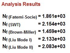
There are several outputs available. First either the fatigue life computed by the various damage models is displayed.
These damage models require a search for the most damaging plane. Results of this search are plotted. There are two possible failure systems. One on planes that are perpendicular to the free surface and shown on the left side of the figure. The angle θ is the angle that a crack would be observed on the surface relative to the σx direction. The second failure system occurs on planes oriented 45° to the surface. Both in and out-of-plane shear stresses must be considered on this plane. These planes are shown on the right side of the diagram. Theta may take on any value on the surface. The shear stress τA is an in-plane shear stress and causes microcracks to grow along the surface. The maximum out-of-plane shear, τB occurs on a plane that is oriented at 45° from the free surface and causes microcracks to grow into the surface.
Results from the SWT calculations are plotted as a function of the angle θ and the expected fatigue life will be the minimum life. The maximum fatigue damage for this model will always occur on a plane that is perpendicular to the free surface so that the 45° plane need not be considered.
Next plots from the three shear stress failure planes are given. The expected fatigue life is the minimum from any of the three shear stresses.
Various stress-strain plots are produced. This data is also available in a tab delimited format for use with the clipboard or file.
Finally, all of the input data is given in a table.