- Fatigue Technologies
- Constant Amplitude
- Fatigue Calculators
- Finders
- Technical Background
- Variable Amplitude
- Finite Element Model
- Multiaxial
- Probabilistic
- High Temperature
- Welded Structures
- Cast Iron
- Small Defect √ Area
- Utilities
- Languages
 日本語
日本語eFatigue gives you everything you need to perform state-of-the-art fatigue analysis over the web. Click here to learn more about eFatigue.
Constant Amplitude Strain-Life Technical Background
The strain life method had its major development during the 1960's. It is based on the premise that the local stresses and strains around a stress concentration control the fatigue life. Although most structures and machine components have nominal stresses that remain elastic, occasional high loads and stress concentrations cause plastic deformation around notches. Fatigue damage is dependant on the local plastic strains around stress concentrators.
The local plastic strains are controlled by the elastic deformation of the surrounding elastic material. Even though external loads are applied, the local region is strain or deformation controlled. The strain resistance of the material is a better measure of the fatigue performance than the stress resistance.
Material Properties
Strain controlled tests are always conducted in axial loading. Deflections are controlled and converted into strain. The resulting forces are measured to compute the applied stress. Metals undergo transient behavior when they are first cycled.
In this example the material becomes stronger with each loading cycle into the plastic range. Other materials loose strength when they are repeatedly plastically deformed. After the initial transient behavior most materials have steady state behavior described by the hysteresis loop. During the fatigue test the strain range, Δε, is controlled and the resulting stabilized stress range, Δσ, is recorded along with the cycles to failure. In strain life testing cycles to failure is converted to reversals to failure. One cycle has two reversals and a symbol 2Nf is used.
Before plotting the strain vs. fatigue life, the total strain that was controlled during the test is divided into the elastic and plastic part. The elastic strain is computed as the stress range divided by the elastic modulus. Plastic strain is obtained by subtracting the elastic strain from the total strain.
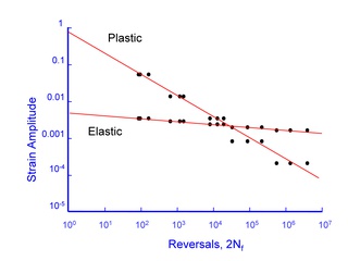
Test data is then fit to a simple power function to obtain the material constants; fatigue ductility coefficient, ε'f , fatigue ductility exponent, c , fatigue strength coefficient, σ'f , and fatigue strength exponent, b.
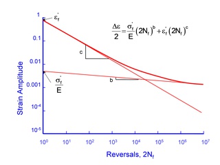
The total strain is then obtained by adding the elastic and plastic portions of the strain to obtain a relationship between the applied strain and the fatigue life.
The materials deformation during a fatigue test is measured in the form of a hysteresis loop. After the initial transient behavior the material stabilizes and the same hysteresis loop is obtained for every loading cycle. Each strain range tested will have a corresponding stress range that is measured. The cyclic stress strain curve is a plot of all of this data.
The cyclic stress strain curve describes the behavior of the material after it has been plastically deformed in service a few times. You can think of the traditional stress strain curve as describing the behavior of the material as it was manufactured. A simple power function is fit to this curve to obtain three material properties; cyclic strength coefficient, K' , cyclic strain hardening exponent, n' , and elastic modulus, E.
Surface Finish Effects
Materials, as they are tested, are always in a different surface condition than the materials as they are actually used. Test specimens are polished to eliminate the effects of surface finish. Fatigue cracks usually nucleate on the surface so that the condition of the surface plays a major role in the fatigue resistance of a component, but only at long lives. At short lives cyclic plasticity dominates the behavior of the material and surface finish is less important. The degree of surface damage depends not only on the processing but also on the strength of the material. Higher strength materials are more susceptible to surface damage. An important part of the analysis is to "correct" the basic materials data to obtain an estimate of the fatigue life of the material in the component or structure of interest. To account for this in the analysis the material fatigue limit is reduced by a surface finish factor, kSF.
The original data for constructing this curve is shown below. The factors tend to provide conservative estimates for fatigue lives.
(From Noll and Lipson, "Allowable Working Stresses", Society for Experimental Stress Analysis, Vol. III, no. 2, 1949)
These data are fit to a simple power function to obtain an estimate of the surface factor for any hardness steel.

| α | β | |
| Ground | 1.58 | -0.085 |
| Machined | 4.51 | -0.265 |
| Hot Rolled | 57.7 | -0.718 |
| Forged | 272 | -0.995 |
The effect of surface finish is reduced for higher strain levels where cyclic plasticity controls the behavior. Surface finish won't have any effect on the static strength of the material ( 1 reversal ).
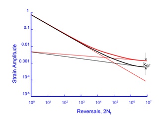
Surface finish effects are included in the analysis by altering the slope of the elastic portion of the strain-life curve. The surface finish corrected slope is given by
It is important to note that this correction should be done after the cyclic strength properties are determined.
Stress Concentrations
Stress concentrations are one of the most important factors affecting the fatigue life of any component or structure. These stress concentrations may be intentional in the design or unintentional such as deep machining marks or other processing related flaws. It seems reasonable to directly compare the maximum stress at a stress concentration to the fatigue limit estimated for that component.
(From MacGregor and Grossman, "Effects of Cyclic Loading on Mechanical Behavior of 24S-T4 and 75S-T6 Aluminum Alloys and SAE 4130 Steel", NACA TN 2812, 1952)
The notched bar in this data has a stress concentration factor Kt of 3.1 and the effect of this notch should reduce the allowable nominal stress amplitude at any fatigue life by an amount equal to Kt. All of the test data lie above this estimate. The effective stress concentration in fatigue is less than the stress concentration factor, Kt. This reduction factor is called the fatigue notch factor, Kf, but it is best thought of as the effective stress concentration in fatigue. The variation between Kf and Kt is dependant on the size of the notch and strength of the material. A material that is very sensitive to notches will have Kf = Kt. A notch sensitivity factor, q, is introduced to quantify this effect.
(From Peterson "Notch Sensitivity", Metal Fatigue, Sines and Waisman, McGraw Hill, 1959)
Smaller radii are less effective in fatigue than larger ones. Fatigue notch factors can be computed from Kt and q.
Peterson fit the available test data for steel and aluminum to obtain an expression for Kf in terms of ultimate strength, Su, and notch radius, ρ in mm.
The stress concentration, Kt or Kf, describes the elastic deformation around a notch. But in the strain approach, the plastic strains must be determined. Neuber's rule is used to convert an elastically computed stress or stain into the real stress or strain when plastic deformation occurs. For example, we may compute a stress with elastic assumptions at a notch to be KtS and this stress exceeds the strength of the material. The real stress will be somewhere on the materials stress-strain curve at some point σ.
Neuber's rule states, with some mathematical proof, that the product of nominal stresses and strains ( S and e ) is proportional to the to the product of the local elastic plastic stresses and strains ( σ and ε ). Mathematically this is expressed as
Nominal strains are computed from the nominal stress from the cyclic stress strain curve before computing the local stress and strain . Nominal stresses and strains can be either elastic or elastic-plastic with this formulation.
A special formulation is used when the nominal stresses and strains come from elastic calculations even though the real stresses may be above the yield strength. Examples include input from elastic finite element models and strength of materials calculations such as bending beams. In this case, Neuber's rule is written in terms of only the applied nominal stress.

In cyclic loading the stress is replaced by the stress amplitude resulting in the more commonly used form of Neuber's rule.
This expression is then combined with the materials cyclic stress strain curve to compute the stress at the notch root Δσ. Once Δσ is known, Δε can be directly computed from the cyclic stress strain curve.
Mean Stresses
Tensile mean stresses are known to reduce the fatigue strength of a component. Compressive mean stresses increase the performance and are frequently used to increase the fatigue strength of a manufactured part. The Smith-Watson-Topper (SWT) parameter is used to account for the effect of mean stresses in the strain approach. The major variables are the maximum stress, σmax, and strain range, Δε, of the stable hysteresis loop.
The strain range provides the driving force for growing small micro cracks and the higher the maximum stress the easier it is for these micro cracks to grow. They proposed a simple damage parameter, PSWT, of
Any combination maximum stress and strain range of that has the same PSWT will have the same fatigue damage. A loading cycle with high maximum stress and small cycles strain ranges can do as much damage as a cycle with low maximum stresses and high cyclic strains. The SWT damage parameter can be related to the constant amplitude material properties generated without a mean stress. In a materials test the maximum stress is equal to the stress amplitude for the zero mean stress strain range.
This expression requires an iterative solution because the stress range, Δσ, is a complex function of 2Nf.
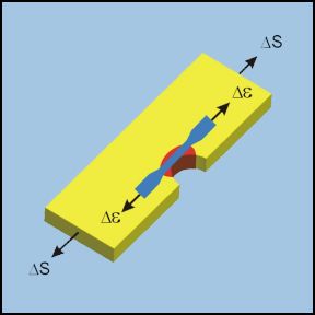
Fatigue damage is dependant on the local stresses and plastic strains around stress concentrators. Local mean stresses can be larger or smaller than the nominal mean stress depending on how much plastic deformation occurs around the stress concentration. Local stress strain response for nominal zero to tension loading is shown below. The maximum stress in the hysteresis loop will always be on the materials cyclic stress strain curve shown by the blue line in the figure.
The local strain range increases with an increase in the nominal stress range as shown by the two hysteresis loops in the drawing. Compressive stresses are formed around the stress concentration upon unloading even though the external nominal stresses were all in tension. Local mean stresses do not increase because the maximum stress is on the flat portion of the cyclic stress strain curve.
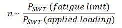
Safety Factor
An approximate safety factor, n, is computed when the combination of the strain range and mean stress is below the fatigue limit of the material. It is computed from PSWT at the fatigue limit of the material.