eFatigue gives you everything you need to perform state-of-the-art fatigue analysis over the web. Click here to learn more about eFatigue.
Multiaxial Stress-Life Technical Background
Fatigue occurs on the surface where one of the principal stresses is usually zero. As a result, multiaxial fatigue problems are usually biaxial in nature. Here we have assumed that the stress normal to the free surface is zero in all the calculations. Any stress concentration effects must be included in the input loading data.
Multiaxial Fatigue Calculators are used for constant amplitude loading where the largest cycle is assumed to do all of the fatigue damage. The Multiaxial Fatigue Analyzer counts cycles and sums fatigue damage for all cycles. More damage models are available with the Multiaxial Fatigue Calculators. Fatigue Analyzers have the ability to read data from files.
Variable amplitude multiaxial stress life analysis can be summarized as a series of steps:
- define applied stresses
- select material properties
- correct material properties for surface finish
- compute fatigue damage
- search for possible failure planes
Go to the Constant Amplitude Technical Background section for a more complete description of the fatigue variables.
Loading
First, loading units must be specified. You can select either stress or strain units from the list.

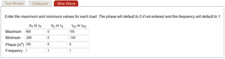
Loading histories can be entered in a series of text boxes, from the clipboard or as sine waves by selecting the appropriate tab. The individual points are connected with straight lines to obtain the loading history. If the second column is left blank, the stress σy is assumed to be zero. The stress is assumed zero even when the other columns have been entered as strain.
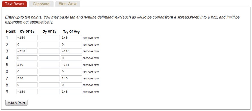
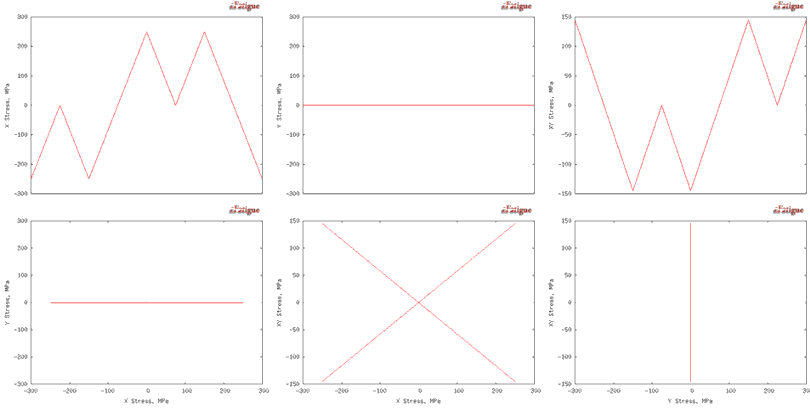
You can view the history with the Plot function. The input data shown above generated the following loading histories. Stresses as a function of time are displayed on the top row. Cross plots between the various stresses are shown in the second row.
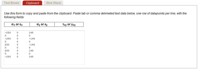
Data entered in text boxes is also available on the Clipboard tab. In this mode, data can be copied from the clipboard or pasted to the clipboard.
Loading histories may also be entered as a series of sine waves. The default frequency is 1 and the default phase is 0o. The frequency is a relative frequency between the various stresses or strains. Here is an example.
Damage Models
There are many damage models used for multiaxial fatigue analysis. We have implemented some of the most common and useful methods including Findley, Sines, Goodman and Dang Van.
A common feature of many stress based multiaxial fatigue criteria is that they are expressed as a general form that includes both shear stress amplitude τa and normal stress σn during a loading cycle. Multiaxial fatigue models differ in the interpretation of how the shear stress amplitude and normal stress are defined. One of the fundamental problems is to evaluate the effective amplitude and mean values of the shear/normal stresses on a material plane.
Fatigue cracks begin on or near the surface. On the surface the stress state is one of plane stress so that there are only three stress components σx, σy and τxy. All other stressses are zero. For these stress states, the accumulation of fatigue damage that will eventually lead to fatigue cracks will occur on planes that are oriented either 45° or 90° to the free surface.
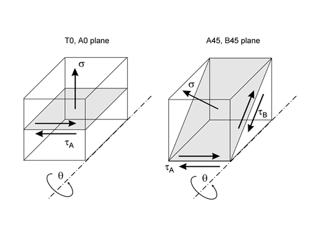
The normal stress is easy to evaluate on any plane. Its direction is fixed and the magnituude varies. But the shear stress can vary in both magnitude and direction. There are two shear stresses acting on the 45° plane. An in-plane stress, τA and an out-of-plane shear stress τB. How should these two shear stress be combined? One possibility is to consider both shear stresses separately because only one of the two slip systems will be activated in an individual grain of the material.
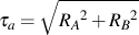
Minimum Circumscribed Ellipse
de Freitas M., Li B, Santos JLT. Multiaxial Fatigue and Deformation: Testing and Prediction, 2000, ASTM STP 1387
An example of the MCE is shown below.
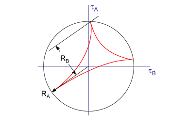
First, the shear stress loading history is determined for a plane. For proportional loading this will always be a straight line. Nonproportional loading histories will have some complex shape. In this case, the the major axis of the ellipse is defined as the smallest circle that will contain all of the shear stresses. This is denoted RA in the example. Using the major axis as a reference, the minor axis, RB is defined as the maximum distance of any stress point in the loading history from the major axis. An equivalent shear stress is then used in the fatigue calculations. This shear stress may be used with any damage model.
Findley
Findley, W. N., "A Theory for the Effect of Mean Stress on Fatigue of Metals Under Combined Torsion and Axial Load or Bending," Journal of Engineering for Industry, Nov. 1959, 301-306
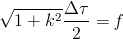
Findley reviewed much the same experimental data as Sines but came to a slightly different model. He suggested that the normal stress σn, acting on a shear plane might have a different linear influence on the allowable alternating shear stress, Δτ/2.
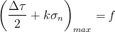
Parabolic forms were investigated but Findley concluded that the linear form was sufficient to describe the experimental data. Here k is a material constant that is related to the materials' sensitivity to normal stresses and f is directly related to the materials' fatigue strength.
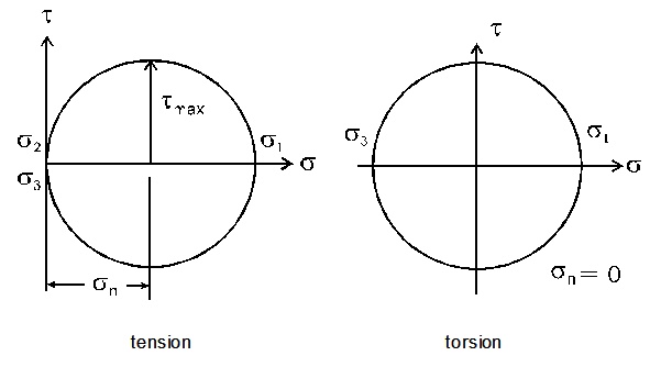
Mohr's circle for both tension and torsion are show below. Both loading conditions have the same shear stress. In an R= -1 fatigue test, both tension and torsion loading will have the same shear stress range acting on a small microcrack located on maximum shear stress plane. But Mohr's circle shows that tension loading will also have a normal stress cycle with the same range as the shear stress acting on this shear plane. The result is that for the same shear stress range, tension loading will always be more damaging than torsion.
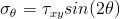
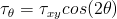
Findley's model differs from Sines' or other yield criteria models in that it identifies the stress acting on a specific plane within the material. These are termed critical planes and can be defined as one or more planes within a material subject to a maximum value of a damage criterion. Fatigue life is controlled by the combination of stresses and strains acting on a critical plane. Findley identifies a critical plane for fatigue crack initiation and growth that is dependent on both alternating shear stress and maximum normal stress. The combined action of shear and normal stresses is responsible for fatigue damage and the maximum value of the quantity in parentheses is used rather than the maximum value of shear stress. This concept is easily illustrated for torsion loading. The stresses σθ and τθ on a plane oriented at an angle θ can be computed from the applied shear stress τxy as
Values of τθ + kσθ for a value of 0.3 are plotted below and failure is expected to occur on the plane that has the largest combination of Δτ/2 + kσn.
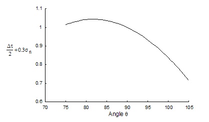
Findley criterion for torsion
The maximum value of the parameter occurs at angles of about 82° and -8°. In the case of pure torsion, it can be shown that Eq. 5.7 becomes
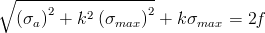
and for pure bending or axial loading with a stress amplitude σa and maximum stress σfgbmax
The constant k is determined experimentally by performing fatigue tests involving two or more stress states. Examples of solutions for k based on the ratio of fatigue strength for two stress states are given below.
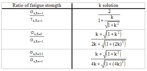
For ductile materials, k typically varies between 0.2 and 0.3.
The Findley criterion is often applied for the case of finite long-life fatigue. An equation of the form
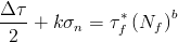
is used where tf* is computed from the torsional fatigue strength coefficient, tf', using
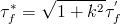
The correction factor
 typically has a value of about 1.04.
Sines
Sines, G., "Behavior of Metals Under Complex Static and Alternating Stresses," in Metal Fatigue, G. Sines and J.L. Waisman. Eds., McGraw Hill, 1959, 145-169.
Sines considered the experimental data of Gough for combined bending and torsion loading. After studying several failure criteria including both maximum shear stress and octahedral shear stress he proposed that the octahedral shear stress be used as a fatigue damage criteria. The physical significance of the octahedral shear stress is that it expresses the average effects of slippage on different planes and in different directions of all crystals in the aggregate with slip in any given grain caused by the critical resolved shear stress in that grain. He notes that
"The scanty existing data do not give grounds for distinguishing whether the maximum shear stress criterion or the octahedral shear stress criterion best fits the experimental results. Moreover, the constants can be chosen so that the two criteria do not differ by more than 8 percent. Both sets of data indicate that alternating shear stress causes the fatigue damage, the difference being caused only by the degree of averaging and by mutual constraint of the crystals. On the basis of present experimental knowledge, then, either criterion can be justifiably applied, the only evident choice between them is the convenience of the mathematical expression in any given case."
In a three dimensional stress state it is more difficult to compute the maximum shear stresses because a cubic equation must be solved for the three principal stresses. Octahedral stresses can be obtained from direct computations using the six stress components for any coordinate system.
To establish the effects of mean stresses, Sines reviewed much of the experimental data for combined bending and torsion tests and grouped the experimental results as follows:
- cyclic axial with static tension and compression,
- cyclic torsion with static torsion,
- cyclic bending with static torsion, and
- cyclic torsion with static bending.
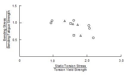
The effect of a static tensile or compressive stress on axial fatigue strength is shown below. The relationship is linear as long as the maximum stress during a cycle does not exceed the yield strength of the material. This is essentially a Goodman diagram. The different symbols represent various materials.
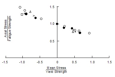
Cyclic axial stress with static tension and compression
Next Sines considered the effect of static torsion on the torsional fatigue strength. The torsional mean stress clearly has no effect on fatigue as long as the maximum shear stress remains below the yield strength of the material. There is no physical significance to the sign of the shear stress. It is used to distinguish between clockwise and counter clockwise rotations.
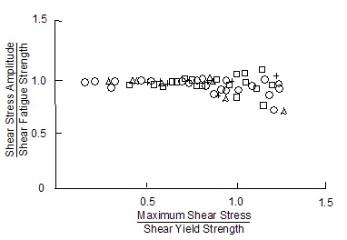
Cyclic torsion with static torsion
The effect of static torsion on reversed bending tests was then considered. Only a limited quantity of data for this stress state was available to Sines, but he concluded that a torsional mean stress did not effect the fatigue limit in bending until the torsional yield strength was exceeded by at least 50 percent.
Cyclic bending with static torsion
The few test data showing the effect of static tension superimposed on alternating torsion suggest a linear dependence between the amplitude of alternating torsion and the static tensile stress.
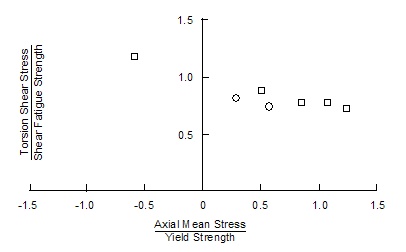
Cyclic torsion with static tension and compression
Because static torsion was not observed to influence either cyclic bending or cyclic torsion fatigue limits and because static tension and compression linearly influenced the fatigue limits in both tension and torsion, Sines concluded that the mean hydrostatic stress, σh, during a cycle had an effect on fatigue life. His resulting failure criterion can be expressed as:
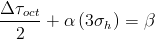
or in terms of the individual stress components as

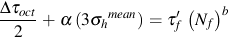
Sines' formulation has the advantage that it is easily solved for complex stress states and only relatively simple tests must be done to determine the two constants α and b. Tests for two mean stresses are needed to determine the constant α.
In the finite life regime the constant β is replaced by a stress life curve where the stresses are plotted in terms of the octahedral shear stress.
Sines method is not very accurate for loadings that have rotating principal stresses.
Goodman
The traditional Goodman diagram can be used with the principal stresses to evaluate fatigue under multiaxial loading. Care must be taken when using principal stresses for loading which involves both tension and compression. The principal stresses and their directions are shown below for both tension and compression loading.
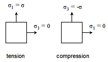
By convention, the principal stresses are always ordered so that σ1 >= σ2 >= σ3. Note that during a simple tension compression loading the principal stress direction rotates 90°. To avoid these problems, the normal stresses are computed for each plane and the range of normal stress acting on a plane is used to compute fatigue lives. The Goodman correction is used to account for mean stresses on each plane. The plane with the lowest fatigue life is considered the critical plane.
Dang Van
Dang-Van, K., "Macro-Micro Approach in High-Cycle Multiaxial Fatigue," in Advances in Multiaxial Fatigue, ASTM STP 1191, D.L. McDowell and R. Ellis, Eds., American Society for Testing and Materials, Philadelphia, 1993, 120-130.
Dang Van has proposed an endurance limit criterion based on the concept of microstresses within a critical volume of the material. This model arises from the observation that fatigue crack nucleation is a local process and begins in grains that have undergone plastic deformation and form characteristic slip bands. It is hypothesized that because cracks usually nucleate in intragranular slip bands, the microscopic shear stress on a grain must be an important parameter. In the same way, it is reasoned that the microscopic shear stress on a grain must be an important parameter. In the same way, it is reasoned that the microscopic hydrostatic stress will influence the opening of these cracks or slip bands. The simplest failure criterion involving these two variables is a linear combination
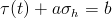
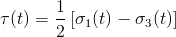
where τ(t) and σh(t) are instantaneous microscopic shear stress and hydrostatic stress and a and b are constants. The constant b is the fatigue strength determined from a torsion test and a is related to the sensitivity of the material to hydrostatic stress.
The microscopic stresses and strains within critical grains are different from the macroscopic stresses and strains commonly computed for fatigue analysis. Two size scales have been distinguished in the model:
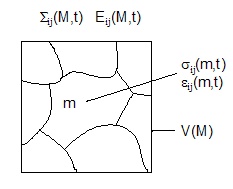
Macroscopic and microscopic scales.
- A macroscopic scale is characterized by an elementary volume V(M) surrounding a point where the fatigue analysis is to be performed. This size scale is on the order of a strain gage or FEM element. This is the scale considered by engineers and is the same as local stresses and strains as defined in the "local strain" approach to fatigue analysis. Macroscopic stresses are denoted Σ(M,t) and strains Ε(M,t). They are both functions of position within the structure, M, and time, t.
- A microstructural scale on the order of a grain or other suitable microstructural unit corresponding to a subdivision of V(M). Microscopic stresses σ(m,t) and strains ε(m,t) are related but not equal to Σ(M,t) and Ε(M,t).
At the microstructural scale, a material is neither isotropic nor homogenous and the values σ(m,t) and ε(m,t) will be different from the local macroscopic variables Σ(M,t) and Ε(M,t). Plastic shear deformation of the grains with the most severe orientations is constrained due to the elastic behavior of neighboring grains having less severe orientations. If fatigue failure is to be avoided, the stresses and strains in the critically oriented grains must stabilize by the process of elastic shakedown and thus prevent crack growth to the neighboring grain.
Computation
of the elastic shakedown state under multiaxial loading is illustrated with the
help of the following figure. The initial elastic domain of the critical
volume of material is illustrated by the circle Co, with center at Oo
and radius Ro. As loading pregresses the material undergoes
combined kinematic and isotropic hardening as the center of the yield surface
translates and the radius of the surface increases. After several
repetitions of the load path, a stable domain CL with center OL
and radius RL will evolve. The stable path is characterized by
the smallest circle, CL that completely encloses the load path.
The stabilized residual stress tensor, r*,
corresponds to OL - Oo. For tension-torsion loading the
domain CL corresponds to a circle in
 stress space but in the general loading case where all six stress components change,
the domain CL is a six dimensional hypersphere.
stress space but in the general loading case where all six stress components change,
the domain CL is a six dimensional hypersphere.
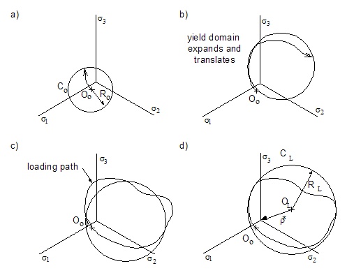
Elastic shakedown under multiaxial loading
Computationally, a combined isotropic and kinematic cyclic plasticity model is used to obtain an estimate of the microscopic stresses acting on the critical grain. Evaluation of the microscopic residual stresses that arise from the combined isotropic and kinematic hardening tensor r* is a critical part of this model and distinguishes it from the other stress based models.
The resulting microscopic stresses, σij, are obtained from the macroscopic stress microscopic residual stresses
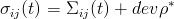
where dev ρ* is the deviatoric part of the stabilized residual stress tensor.
The microscopic shear stress which is used in the failure criterion is computed from the microscopic principal stresses at every point in the loading cycle using the Tresca maximum shear stress theory.
The failure criterion can then be expressed as combinations of t(t) and hydrostatic stress. The constants a and b are obtained from materials tests at two different stress states. A loading path that remains within the two bounding failure lines is expected to have infinite life while any path that extends outside the damage line will have fatigue failures because microscopic plastic strains occur.
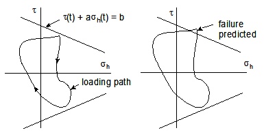
Dang Van criteria.
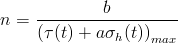
The Dang Van criterion is intended as a method of predicting the endurance limit under complex loading situations. Unlike the other methods, the output from the analysis is always expressed as a safety factor not a fatigue life. It is computed as
Materials
This section describes how material properties are estimated from limited input data. The minimum input data required is the type of material, steel or aluminum, and the ultimate strength. All other properties can be estimated or calculated.
Elastic Properties
Estimated:
| Elastic Modulus, E |
207,000 MPa for Steel 80,000 MPa for Aluminum |
| Poisson's Ratio, n | 0.3 |
| Shear Modulus, G |  |
Tensile Stress Life Curve
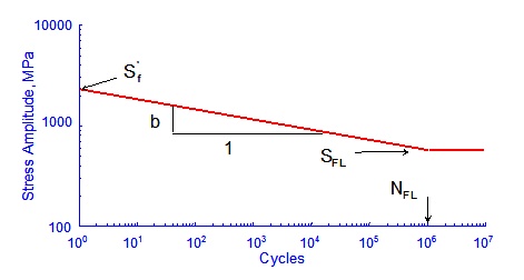
The stress life curve is described by four properties; fatigue limit, SFL, fatigue limit cycles, NFL, intercept at 1 cycle, Sf', and slope, b. Various approximations are made depending on which material properties are specified.
Four properties specified
Only three of these properties are independent. If all four are specified, the fatigue limit is ignored and recalculated to be consistent with the other properties.
Three properties specified
When any three properties are known, the remaining one is calculated directly.
A default value of NFL =106 cycles is assumed if the slope and intercept is specified. The fatigue limit is then computed.
A default slope of -0.085 is assumed when only the fatigue limit and fatigue limit cycles is specified. The intercept is then computed.
One property specified
A default value of NFL = 106 is assumed. When either the fatigue limit or stress life intercept is entered, a slope of -0.085 is assumed and the other property is calculated.
No property specified
Lacking other data, these constants are estimated from the Ultimate Strength, Su.
| Stress Life Intercept, Sf' | Sf' = 1.62 Su |
| Fatigue Limit, SFL | SFL = 0.5 Su |
| Stress Life Slope, b |  |
| Fatigue Limit Cycles, NFL | NFL = 106 |
Torsion Stress Life Curve
Torsion stress life curves can be formulated in terms either maximum shear stress or octahedral shear stress. First, any properties that are specified are used. Lacking test data, these properties are estimated from the tensile stress life curve constants that have been determined above.
Fatigue limit cycles, NFL, is assumed to be the same for both tension and shear, and a separate property is not defined.
Maximum Shear Stress
Findley's model is assumed to be valid for converting tensile data into maximum shear stress data. The ratio of shear to tensile properties depends on the constant k in Findley's model.
This correction factor, CF, typically varies from 1.2 to 1.5
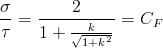
| Maximum Shear Intercept, Tf'max | Tf'max = Sf' / CF |
| Maximum Shear Slope, bmax | bmax = b |
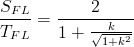
| Maximum Shear Fatigue Limit, TFLmax | TFLmax = SFL / CF |
Octahedral Shear Stress
Properties in terms of octahedral shear stress, τoct, can be computed from the tensile properties.

| Octahedral Shear Intercept, Tf'oct | Tf'oct = Sf' * 0.47 |
| Octahedral Shear Slope, boct | boct = b |
| Octahedral Shear Fatigue Limit, TFLoct | TFLoct = SFL * 0.47 |
Findley Model Constants
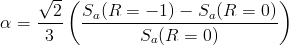
The Findley constant, k, is computed from the ratio of tensile and shear fatigue limits when these properties are specified.
In the absence of test data, a default value of 0.3 is assumed.
Sines Model Constants
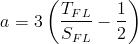
The constant a in Sines' model is computed from mean stress data.
In the absence of test data, a default value of 0.15 is assumed.
Dang Van Model Constants
The Dang Van constants are computed from the tensile and torsion fatigue limits.

In the absence of test data, a default value of 0.4 is assumed for a.
Surface Finish Effects
Modifying factors entry and defaults are the same as constant amplitude analysis. Go to the Constant Amplitude Technical Background section for a more complete description.
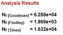
Output
There are several outputs available. First either the fatigue life or safety factor computed by the various damage models are displayed. A safety factor of < 1 for Dang Van means that failures are likely.
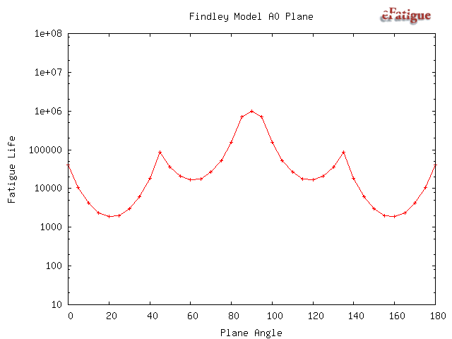
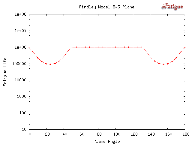
The Findley damage model requires a search for the most damaging plane. Results of this search are plotted. There are two possible failure systems. One on planes that are perpendicular to the free surface and shown on the left side of the figure. The angle θ is the angle that a crack would be observed on the surface relative to the σx direction. The second failure system occurs on planes oriented 45° to the surface. Both in and out-of-plane shear stresses must be considered on this plane. These planes are shown on the right side of the diagram. Theta may take on any value on the surface. The shear stress τA is an in-plane shear stress and causes microcracks to grow along the surface. The maximum out-of-plane shear, τB occurs on a plane that is oriented at 45° from the free surface and causes microcracks to grow into the surface.
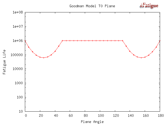
Results from the Goodman calculations are plotted as a function of the angle θ and the expected fatigue life will be the minimum life. The maximum fatigue damage for this model will always occur on a plane that is perpendicular to the free surface so that the 45° plane need not be considered.
Next plots from the three shear stress failure planes are given. The expected fatigue life is the minimum from any of the three shear stresses.

Finally, all of the input data is given in a table.