
eFatigue gives you everything you need to perform state-of-the-art fatigue analysis over the web. Click here to learn more about eFatigue.
Probabilistic Statistical Simulations Technical Background
Probabilistic modeling is based on a statistical simulation of a deterministic model. The deterministic variables in a traditional fatigue calculation are replaced by random variables. Each of these random variables is described by a statistical distribution. Given the input distributions, probabilistic analysis is employed to find the output distribution, in the case, the distribution of fatigue lives. This process is illustrated below for the simple case of stress and strength. Failure occurs whenever stress is greater than the strength.
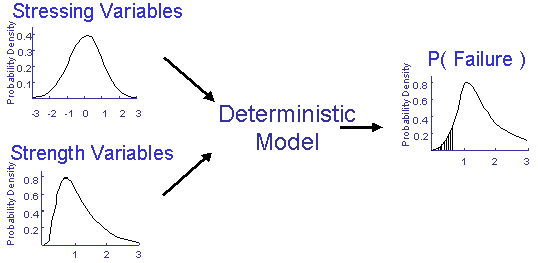
There are many techniques available to do the simulation. One of the simplest is the Monte Carlo method. A value of the strength is randomly selected from its statistical distribution and compared to a randomly selected value of the strength. The selection is random but must be taken from the underlying statistical distribution of the variable of interest. This process is repeated hundreds or thousands of times and the number of failures is tabulated. The probability of failure for this simple example is simply the number of failures divided by the total number of trials. In statistical simulations the traditional deterministic variables in a mathematical model are replaced with random variables.
Statistical simulation involves three major steps:
- Generate random variables,
- Compute fatigue life for each set of variables,
- and Evaluate probabilistic sensitivity coefficients.
Generating Random Variables
Sampling or generating random variables from any statistical distribution can be done with the cumulative distribution function ( CDF ). The CDF is the probability that X will be less than or equal to a value of x.

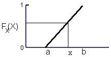
The CDF ranges from 0 to 1 which provides a convenient method for generating variables with any known statistical distribution. Any value of the CDF has the same probability of occurrence just like any single sample of a variable in the analysis.


Start with a random number between 0 and 1 called RAND. Any value of RAND has the same probability of occurrence. Then transform it with the CDF into the variable of interest.
Transformation for a uniform distribution with a location parameter mx and scale parameter s proceeds as follows. The location parameter is the mean value

and the scale parameter, s, is computed from the limits a and b.

Individual values, each with the same probability of occurrence, of the random variable x can be obtained from this expression.

Generating normal variables is slightly more complex due to the mathematical nature of the cumulative distribution function. Consider a normal distribution with mean mx and standard deviation sx. The random variable x can be obtained from the following expression where z is the standard normal deviate with a mean of 0 and standard deviation of 1.

A random number is generated and treated as the probability in standard normal tables denoted F

For example the random number 0.8413 would be transformed into the normal deviate z = 1.0 or one standard deviation. Normal variables can easily be obtained in EXCEL using the NORMINV worksheet function.
Log-Normal distributions are generated from the same expressions where the normal variables are replaced by the logs.
A Gumbel extreme value distribution is generated from the scale parameter a and location parameter b as and a random number RAND follows

Weibull distributions are generated from the scale parameter b and Weibull slope c

Correlated Variables
There is usually a strong correlation between slopes and intercepts in the various material properties employed in fatigue analysis. Fatigue data from a large number of fatigue tests is given below. This strain life data is merged from 29 data sets.
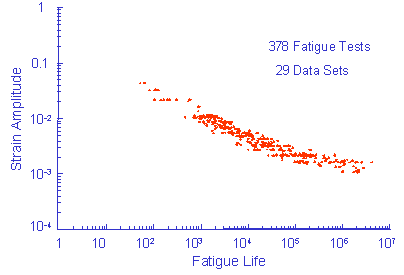
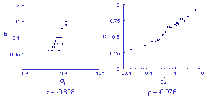
Fatigue constants were fit to the individual data sets to obtain some measure of the variability of the material. The variability in the fatigue strength coefficient and exponent are shown below. The fatigue ductility coefficient and exponent show similar behavior and are adequately described by a Log-Normal distribution.
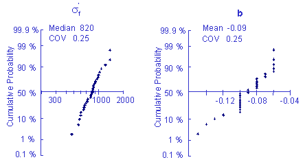
For purposes of illustration this data was used to simulate 100 strain life curves, each one representing same probability of occurrence. The individual fatigue properties are treated as independent random variables.

These curves should provide an estimate of the scatter in the original test data.
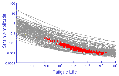
The simulation generates much more variability that the original test data even to the point that the simulation is unreasonable and any results obtained from this simulation would be worthless. This unreasonable simulation is a result of the correlation between the slopes and intercepts shown below. This plot represents the slope and intercept from each of the 29 data sets. High values of the slope always occur with high values of the intercept. Here r is the linear correlation coefficient.
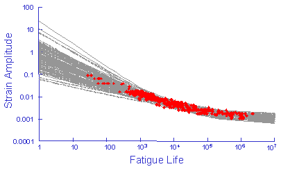
Correlated variables must be considered when doing any statistical simulation. Results from a simulation using correlated variables are shown below. The improvement over the previous simulation is apparent.
Generating two correlated variables is a straightforward process. Consider two normal variables x and y that are correlated with a linear correlation coefficient r. The first step in the process is to obtain two independent standard normal deviates, z1 and z2.


A third correlated normal deviate is then constructed from the first two

The random variables x and y are determined from z1 and z3


Generating correlated distribution between non-normal or mixed distributions follows a similar process. The other distributions are first mapped into a standard linear deviate.
For a Gumbel distribution

and for a Weibull distribution

Monte Carlo Simulation
Each of the variables generated in the simulation process has an equal probability of occurrence. Each combination of variables also has an equal probability of occurrence. One set of variables is just as likely as any other set. The Monte Carlo simulation process simply solves the deterministic model for every set of input variables. A typical set of input variables for the stress life analysis is shown below.
| Smax | Smin | Su | SFL | kSF | Kt |
|---|---|---|---|---|---|
| 179 | -162 | 905 | 258 | 0.71 | 2.99 |
| 156 | -153 | 982 | 232 | 0.70 | 2.94 |
| 224 | -198 | 1107 | 231 | 0.70 | 3.01 |
| 198 | -208 | 1097 | 268 | 0.70 | 3.06 |
| 200 | -203 | 1115 | 250 | 0.71 | 3.06 |
| 188 | -180 | 1180 | 247 | 0.71 | 3.04 |
| 220 | -197 | 1016 | 250 | 0.69 | 2.96 |
| 172 | -208 | 962 | 255 | 0.69 | 2.99 |
| 203 | -200 | 1062 | 252 | 0.69 | 2.91 |
Variables without distributions are treated as constants and no statistical distribution is generated. A typical output from the simulation is shown below. Results are plotted on a Log-Normal probability scale.
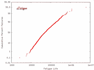
The vertical axis represents the cumulative probability of failure and the estimated fatigue life is plotted on the horizontal sale. Cumulative probability is linear in standard deviations and nonlinear in probability. Each data point represents one of the simulation results. The cumulative probability is obtained by first rank ordering the N results and then computing the cumulative probability for the ith result from

Probabilistic Sensitivity Factors
Sensitivity factors provide information about the relative importance of the variability or uncertainty of all of the input variables and their influence on the resulting fatigue life. Deterministic sensitivity factors Si quantify how a change in the mean will affect the fatigue life. Each variable Xi has its own sensitivity factor.

These are then normalized with the mean values so that they can be directly compared with each other.

Probabilistic sensitivity factors ai are used to quantify the relative effects of variability and uncertainty. For example, the computed fatigue life may be very sensitive to the elastic modulus of the material, but the uncertainty in the elastic modulus is small so that it is not a major contributor to the overall variability in fatigue life.

The alphas are normalized so the sum of their squares equals 1. The results from the simulation are plotted in a pie chart.

In this example, uncertainties or variability in loading contribute to about half of the overall variability.
 日本語
日本語