- Fatigue Technologies
- Constant Amplitude
- Variable Amplitude
- Finite Element Model
- Multiaxial
- Probabilistic
- Fatigue Calculators
- Finders
- Technical Background
- High Temperature
- Welded Structures
- Cast Iron
- Small Defect √ Area
- Utilities
- Languages
 日本語
日本語eFatigue gives you everything you need to perform state-of-the-art fatigue analysis over the web. Click here to learn more about eFatigue.
Probabilistic Strain-Life Technical Background
Strain life analysis can be summarized as a series of steps:
- define applied nominal stress or strain range
- select material properties
- determine stress concentration factor
- use Neuber's rule to compute local stresses and strains
- solve the equations
Go to the Constant Amplitude Technical Background section for a more complete description of the fatigue variables.
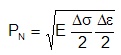
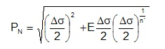
The process starts with determining the local stress, ΔS, and strain, Δe, ranges from the input data. First the Neuber constant PN is computed.
For elastic plastic input, the unknown nominal stress, ΔS, or nominal strain, Δe, is computed from the material's cyclic stress strain curve.
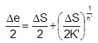
The Neuber constant is directly related to the local stresses and strains.
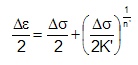
The materials cyclic stress strain curve is employed to compute the local stresses.
Local strains are then computed from the local stresses.
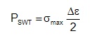
The same procedure is used to determine the maximum local stress, smax. The stress and strain amplitudes in the preceding equations are replaced by the maximum stress and strain.
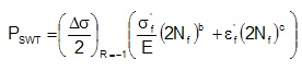
Fatigue lives are then computed from the Smith Watson Topper parameter, PSWT.
Monte Carlo simulation is employed to obtain several estimates of the fatigue life. A random sample for each of the variables is obtained from its underlying statistical distribution and the fatigue life computed. The nature of the equations requires an iterative solution to obtain an estimate of the fatigue life. This process is repeated 100 times to obtain an estimate of the failure probability.
Loading Variability
Statistical distributions can be specified for any of the loading variables. These loading variables are assumed to be statistically independent. Typically there is a strong correlation between these variables. For example, measured strains from a vibrating bracket are shown below. High tension strains are often followed by high compressive strains.
For loading situations like this it is better to enter stress ranges and means than maximum and minimum stresses.
Reasonable values for the minimum and mean stress include zero. This creates a problem in computing the standard deviation from the COV. Whenever either of these variables is zero, enter the standard deviation as the scale factor. Only Normal and Uniform distributions can be used with a zero value.
What is a reasonable variability for the loading variables? Naturally every situation is different but based on past experience we can provide some general guidance. The relationship between standard deviation and COV for a LogNormal distribution is given below. Three standard deviations represent most (99.7%) of the data. Most of the data is within �16% of the median for a COV of 0.05 and within a factor of �2 for a COV of 0.25.
|
COVx |
Standard Deviation Inx |
||
|
1 68.3% |
2 95.4% |
3 99.7% |
|
|
0.05 0.1 0.25 0.5 1 |
1.05 1.10 1.28 1.60 2.30 |
1.11 1.23 1.66 2.64 5.53 |
1.16 1.33 2.04 3.92 11.1 |
When comparing loading histories for determining the variability it is convenient to define an equivalent constant amplitude load from a variable amplitude history. That is what constant amplitude load would produce the same fatigue life as the original loading history? The equivalent load, Feq for 106 constant amplitude cycles can be computed from the loading history as
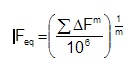
where m is the slope of the SN curve. Typically this should be 4-6 for notched components. Two sets of data are plotted in the figure below. One set of data comes from test track driving of a motor home, the other comes from driving an auto in various cities during normal operation.
Here we are interested in the COV for the two sets of data. The test track data has a COV of 0.12 which is typical of controlled processes. Unsupervised city driving has much more variability with a COV of 0.3.
Selecting an appropriate variability will depend on how well controlled the loading will be. Many customers with widely varying usage characteristics will have a high variability.
Materials
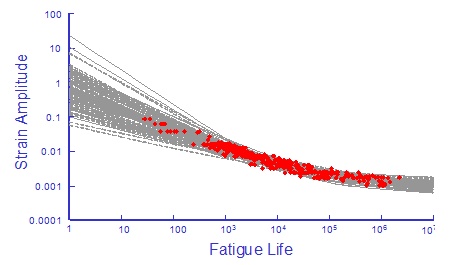
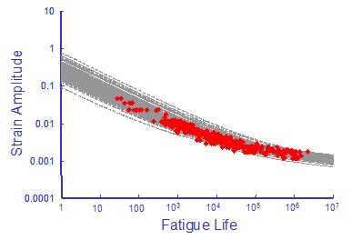
A large number of test data for a sing material 950X, is shown below. The data is a compilation of 29 individual data sets.
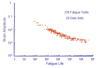
Fatigue constants were fit to all of the individual data sets with the results shown below.
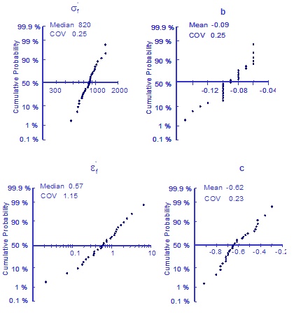
The variability in the elastic modulus is small and is ignored. During the Monte Carlo simulation a value for each of the four material properties will be selected at random and a strain life curve will be constructed.
Results for 100 simulations of this data are shown below.
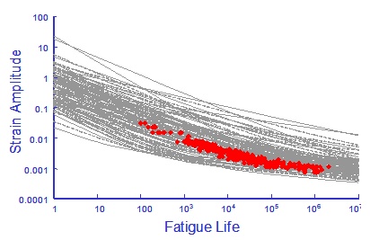
Clearly the results of this simulation are unacceptable because they do not pass through the central tendency of the original test data and they have much more variability. The resulting reliability calculations will be meaningless.
In the preceding simulation each of the variables was assumed to be independent of all other variables. A cross plot of the slopes and intercepts shows a very strong correlation.
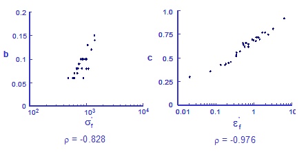
A general observation is that slopes and intercepts for all fatigue data are highly correlated. Provisions have been made to use correlated variables during the simulation.
Adding the correlation coefficients to the simulation produces the following results.
There is considerable improvement in the simulation.
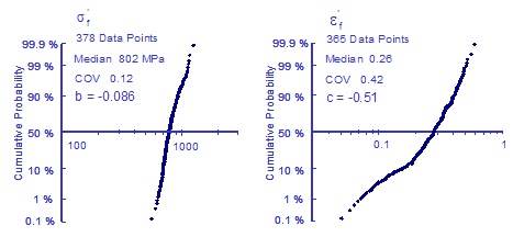
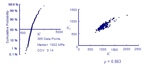
Since there is such a high degree of correlation between the slopes and intercepts it is often convenient to make the slopes constant and put all of the variability into the intercepts. Fatigue constants were fit to all 378 data points to find the best slopes. Using these slopes, the fatigue strength and ductility coefficients were then obtained for each data point to obtain a distribution of the material properties.
This simulation produces the following results.
The preceding examples show the importance of considering correlated variables in the statistical simulation. We should also consider correlation between the fatigue strength and ductility exponents since tensile strength correlates with ductility.
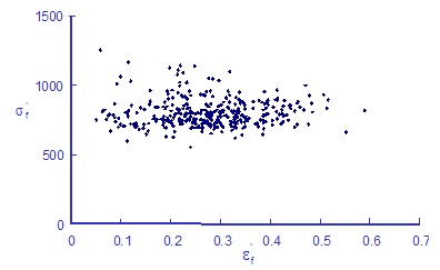
The fatigue strength and ductility do not appear to be strongly correlated. There is, however, a strong correlation between the fatigue strength coefficient and cyclic strength coefficient.
There are two ways to account for this correlation. The statistical distribution and correlation coefficient for the cyclic strength coefficient may be input directly. If the values are left blank the cyclic strength coefficient and strain hardening exponent will be directly computed from the other four fatigue properties so they will be highly correlated.
In the absence of test data, a COV=0.1 or 0.15 for the fatigue strength coefficient and values of 0.2 - 0.4 for the fatigue ductility coefficient are reasonable.
Surface Finish
Surface finish data from an aluminum casting is given below.
Shigley recommends COV's ranging from 0.06 to 0.13 depending on the process.
Stress Concentration
Fatigue notch factors are computed from the stress concentration factors so that the fatigue notch factor will have the same distribution as the stress concentration factor. The variability in stress concentrations will depend on the application. For example, the variability in the stress concentration for a drilled hole will be very small. Here we may estimate a COV=0.05. The variability in a welded joint will be much higher where COVs of 0.2 or 0.3 would be appropriate.
The Simulation
One thousand trials are used in the simulation resulting in 1000 calculated fatigue lives.
Output Results
Results of the simulation are given in graphical and tabular formats. First, the median life from the simulation is given. If the fatigue lives in the simulation are finite, a cumulative distribution of the calculated lives is presented in a LogNormal format. This chart is useful for determining probabilities of failure for other lives. Numerical values for this plot are available as the log of the life and number of standard deviations.
A probabilistic sensitivity analysis is performed to determine which variables have the highest contribution to the variability in fatigue lives. The probabilistic sensitivity factor αi is determined as:
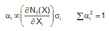
The first term ∂Nf(X) / ∂Xi is the influence of the variable Xi on the fatigue life. This determines the most important variables affecting the fatigue life. It is multiplied by the standard deviation σi. A variable that may have a large influence on the fatigue life may have very little variability so that it will not contribute to the variability in fatigue lives. The elastic modulus is an example of such a variable. Results are plotted in a pie chart.
A table of the sensitivity factors is given. Mean and COV of the distributions used in the simulation are shown in the right side of the table.
A table of results from the simulation is also given. The input data is displayed first. All calculated variables are also given.