- Fatigue Technologies
- Constant Amplitude
- Variable Amplitude
- Finite Element Model
- Multiaxial
- Probabilistic
- High Temperature
- Welded Structures
- Fatigue Analyzers
- BS 7608
- International Institute
of Welding - Aluminum Association
- Strain-Life
- Crack Growth
- Probabilistic BS 7608
- Probabilistic Crack Growth
- VA BS 7608
- VA International Institute
of Welding - VA Aluminum Association
- VA Crack Growth
- Finders
- Technical Background
- Cast Iron
- Small Defect √ Area
- Utilities
- Languages
 日本語
日本語eFatigue gives you everything you need to perform state-of-the-art fatigue analysis over the web. Click here to learn more about eFatigue.
Variable Amplitude Crack Growth Technical Background
All fatigue cracks have very large stress concentrations associated with them. Traditional methods and material properties are not able to describe the behavior of a cracked structure. Instead fracture mechanics is used. Fracture mechanics is a way of computing the stress and strain fields around a crack. For an isotropic elastic material, the stress in the neighborhood of a crack can be easily computed.
Crack Growth calculations may be summarized in these steps.
- define nominal stresses
- select material properties
- determine crack geometry
- specify initial and final crack size
- integrate crack growth equations
Go to the Constant Amplitude Technical Background section for a more complete description of the fatigue variables.
In variable amplitude crack growth, special consideration must be given to the sequencing of the cycles. Crack growth during a loading cycle will depend not only on its magnitude, but also on the magnitude of the loading cycles that preceded it. The figure below shows a crack and the stress fields that surround it at the maximum load in the loading cycle. Real cracks are not microscopically flat and have some texture which is exaggerated in the figure. Behavior of the material near the crack tip can be visualized by imagining the crack path as a series of small material specimens. The stress concentration of the crack results in a large plastic zone in front of the crack with high tensile stresses. Material in this zone is stretched. Because crack the crack is growing, material behind the crack tip has also been stretched during prior loading cycles.
Now unload this crack. The elastic material that surrounds the crack tip outside the plastic zone will force all the displacements near the crack tip back to zero. Because the material element at the crack tip has been stretched, compressive stresses will be required to bring the displacement back to zero. Additional compressive stress must also be added to bring the displacements behind the crack tip to zero since this material has also been stretched. A compressive stress field exists around the crack tip when it is unloaded even though all the external loads were in tension. This process is referred to as crack closure and illustrated below. Residual stresses hold the crack closed.
During subsequent loading these compressive residual stresses must be overcome before the crack can grow again. Cracks can only grow when the crack opens and tensile stresses form at the crack tip. The opening stress is determined by the largest cycle in the loading history. Typically the opening stress is about one third of the maximum load. Portions of the loading history that are above the opening stress will cause crack growth. The portion of the loading history that is below the opening stress will not cause crack growth.
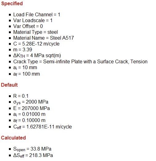
Newman's model is used to make an estimate of the opening stress for a loading history. J.C. Newman "A Crack Opening Stress Equation For Fatigue Crack Growth" International Journal of Fracture Vol. 24, No. 4 , R131- R135, 1984. The opening stress, Sopen , is a function of the maximum stress, Smax , stress ratio, R, yield or flow stress, σys , and constraint factor α. The constraint factor ranges from 1 for plane stress to 3 for plane strain.

Computed opening stresses from these equations for various ratios of Smax/σys are given below for a constraint factor of 2.
The first step in the processing a loading history is to obtain the opening stress. If the loading history has been entered as a time history, the portion of the loading history above the opening stress will be rainflow counted to obtain a histogram of the cycles that will cause the crack to grow. When the loading history has been entered as a rainflow histogram, a new histogram will be computed of only those cycles above the opening stress.
The crack growth calculation starts with the Paris law for constant amplitude loading and written it in terms of effective stress intensity.
An effective crack growth coefficient, Ceff, is obtained from the crack growth coefficient, C.
and

In variable amplitude loading crack growth must be summed for every cycle in the loading history.

This equation is the same as constant amplitude crack growth analysis if the stress range ΔS is replaced with an effective stress range ΔSeq
and C is replaced by Ceff.
Loading History
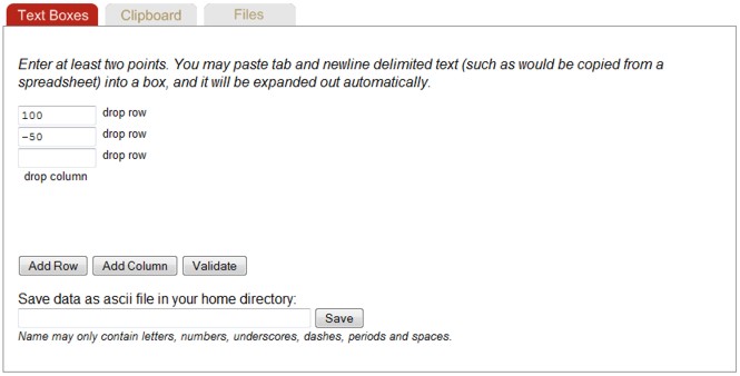
Several methods may be used to input the loading history. These include Text Boxes, Clipboard and Files. Loading data may be either time histories or histograms.
Text Box input may be used to manually enter a loading history. The loading history can contain several channels, one channel per column. Histograms may also be entered. Histograms must be a square matrix in a To-From format with the same number of rows and columns. The first row and column must contain the values for the bin limits. An example of the histogram format can be found in the files section. Supported File Types
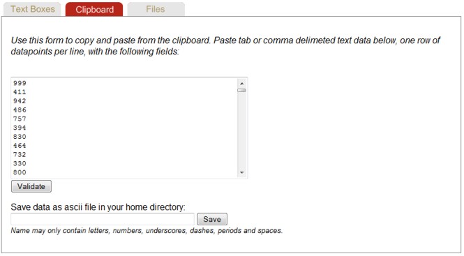
The Clipboard entry is a more convienient way to enter large chunks of data. Data in the clipboard may be edited directly in the clipboard view and is also automatically placed in the text boxes. Similarly, data entered in Text Boxes is available in the clipboard view.
eFatigue supports a number of data file formats. A complete description is found in Supported File Types.
Go to Working With Files if you are unfamiliar with the eFatigue file system.
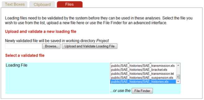
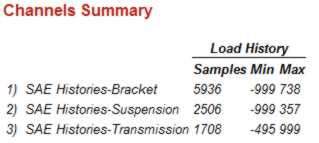
eFatigue uses a file validation process to make sure that the file can be read before conducting any analysis. Key information such as number of channels, maximums and minimums are also obtained from the validation process. This information is always displayed once a file is selected.
Units for the loading history must be selected. The load scale factor defaults to 1 and zero offset to 0 if left blank. Data is scaled as data * scale + offset.
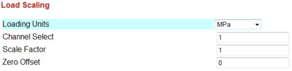
Unscaled data may be plotted with the Plot button.
Materials Data
Most of the materials data and defaults are the same as constant amplitude analysis. Go to the Constant Amplitude Technical Background section for a more complete description. In variable amplitude analysis the yield strength and R ratio for the materials data may also be entered.
Output File
You can specify a filename for the output results in the Output Definition section. A default filename will be assigned if this is left blank.
Analyze
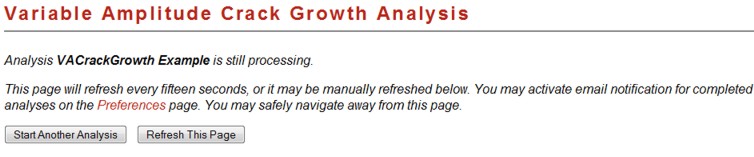
A new window will appear after the Analysis is started. At this point the analysis is sent to a separate server for processing. You may safely navigate away from this window at this point. If you remain on this page, the analysis results will automatically be displayed when completed. Otherwise the analysis results willl be placed in your working directory. For a very long loading history, you may wish to turn on an email notification by going to your Account page.
Results
The fatigue life is given first. The number represents the number of times the entire load history can be repeated, not the total number of cycles.
A plot of the crack length as a function of the number of repeats of the loading history is displayed.
A cumulative exceedance diagram for the cycle ranges is displayed. These diagrams are useful for describing the nature of the loading history and to compare one history with another in terms of stress amplitudes and number of cycles.

Rainflow histograms of the cycles are displayed if the input is a time history. They are displayed in a To_From format. In this format, zero range is along the one of the diagonals and zero mean along the other diagonal.
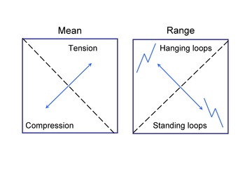
This loading history has a fairly symmetric distribution of hanging and standing cycles. It also has a tensile mean.
The fatigue damage for each bin in the cycle histogram is displayed. Damage for larger cycles will always be more than the damage for an individual smaller cycle. The damage displayed represents the damage for all of the cycles in a bin. In this loading history, most of the damage is done by a small number of high amplitude cycles.
Finally, a listing of all of the input parameters is given with any default parameters that have been used in the analysis.